
Table of Contents
Introduction
This is part 2 of the aquatic food web example. If you haven't finished part 1 of this tutorial, you can use this file. You will find that the pace quickens somewhat in this part, so be sure you have understood the basics of part 1 before you continue.
In this part we first include a model for fish, and then define the three species of fish that inhabit the Glein river (Eel, Perch and Minnow). We examine the time series data for the fish model and reflect on how the fish and invertebrate model could communicate. We consider adding other models, and then do so. Finally, we enter some time series and parameter values, run a simulation and look at the results.
Step 1: Adding a model for fish
 Go to the
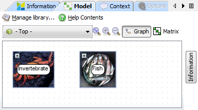
  Model screen and add Food > Aquatic food > Fish from the library. Important: MERLIN-Expo will ask you if you want to connect this model with existing models. For the sake of the exercise, Cancel this action.
Step 2: Add fish species
 Continue to the
  Context tab.
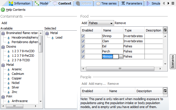
The drop-down list next to the Add button of the Food section should now contain an item named Fishes. Click the  Add button three times to add three species of fish. Name them Eel, Perch and Minnow.
Step 3: Time series data
The listing of time series data should now contain one section for invertebrates and one for fish.
The fish model require river temperature and concentrations, just like the invertebrate model. However, if you have added invertebrates in the context screen, the fish model will ask you for lead concentrations in these. This is because invertebrates are considered a potential diet for fish.
- Hey, stop! you say. Why do I have to enter these concentrations? Shouldn't the invertebrate model calculate them for me?
You are correct of course. Let us return to the model screen.
Step 4: Revisiting the model screen
Return to the model screen.
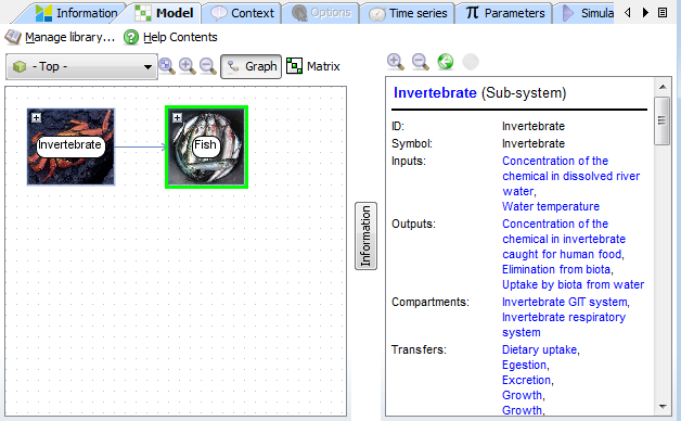
 The information panel allows us to dive into the models and see what their internals look like. Click the Information button located to the right of your graph to reveal the panel. Next click the Fish sub-system. The information panel will now list all the components of the sub-system and you can click each of these items for an explanation. The very first part lists the inputs and outputs for fish. Among the inputs, you will find an input with the long name Concentration of the chemical in invertebrate caught for human food.
Proceed to select the Invertebrate sub-system. Among its inputs/outputs you will find an output with the same name.
 This means that we can connect the Invertebrate model with the Fish model and tell it to provide the Fish model with the concentration data. For this we use a connector:
- Move the mouse cursor to the center of the invertebrate sub-system. A green outline should be displayed.
- Keep the mouse button pressed and move it to the center of the fish sub-system, until you see a green outline around the fish box.
An arrow should now connect the Invertebrate with the Fish model. When you connect two sub-systems, MERLIN-Expo will automatically try to match all inputs of the target with corresponding outputs of the source. To manually set what goes from one sub-system into another, you must edit the connector:
- Right click the arrow
- Select Edit from the menu
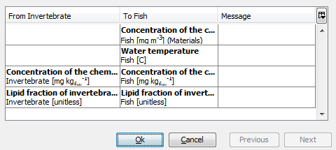 The window lists all potential inputs to the fish model. You should see two outputs of the invertebrate model being fed to the fish model - the lead concentration of invertebrate as well as a parameter you had not even thought about - the lipid content of invertebrates. Thank you MERLIN-Expo.
Go back to the time series screen. The fish model should no longer ask you for chemical concentrations in invertebrates.
Step 5: Adding river
With this revelation fresh in mind, we should think one step further. Both fish and invertebrate models ask us to enter river temperature and lead concentrations. The MERLIN-Expo library contains a river model. Why not use it?
In the model screen, add Environment>Environment>River from the library. MERLIN-Expo will ask you if you want to connect this model with existing models. This time, say yes!
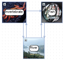 Arrows should now have been added from the river to each model, but also from both fish and invertebrate to the river.
What goes on here? Select each arrow and see what the Information panel says. When clicking on the arrow from River to Fish, we see that River will supply Fish with data on lead concentration and river temperature - this is why we added River.
But why is there an arrow from Fish to River? A click on this arrow reveals that Fish informs River on how much lead is released by fish to the river (via elimination). Fish also tells River how much lead is taken up (removed from the river) by fish.
This can be confusing at first: the arrows between the sub-system boxes do not necessarily indicate a flow of mass (lead) but a flow of information.
Step 6: Time series revisited
Go back to the time series screen. You will be happy to see that the time series required by fish and invertebrates have disappeared. You might be less happy to see the long list of time series required by the river model.
Don't worry. Many of these time series are relevant only for specific processes - wind speed is only needed when there is diffusion of chemicals between air and water, irrigation rate is only interesting when water from the river is used for irrigation, etc.
For the sake of simplicity, we will assume that the Glein is contaminated upstream and disregard any interaction with the atmosphere. This leaves us three time series to enter data for.
For each time series given below, copy-paste the data into the corresponding table (only the data, not the header):
Concentration of the pollutant in raw water entering into the zone of interest from the upstream river zone
Contaminant: Lead
| Time (d) | Value (mg m-3) |
|---|---|
| 0 | 1600 |
Flow rate of the river
This time series emulates a surge in flow rate in March corresponding to spring flooding. Notice that the time series starts at day 0 and ends at day 365 with the same value as for day 0. This makes it possible to re-use the same time series for every year.
| Time (d) | Value (m3s-1) |
|---|---|
| 0 | 50000.0 |
| 80 | 60000.0 |
| 90 | 250000.0 |
| 100 | 100000.0 |
| 270 | 50000.0 |
| 365 | 50000.0 |
Temperature of river water
| Time (d) | Value (C) |
|---|---|
| 0.0 | 2.0 |
| 30.0 | 3.0 |
| 60.0 | 5.0 |
| 90.0 | 9.0 |
| 120.0 | 12.0 |
| 150.0 | 15.0 |
| 180.0 | 17.0 |
| 210.0 | 18.0 |
| 240.0 | 16.0 |
| 270.0 | 13.0 |
| 300.0 | 8.0 |
| 330.0 | 3.0 |
| 365.0 | 2.0 |
Step 7: Parameters
Enter the parameters screen. The list of parameters have grown considerably since your last visit.
Update the following parameters:
Fish
Fish age at maturity
| Fishes | Value | Unit |
|---|---|---|
| Eel | 9125 | d |
| Perch | 1270 | d |
| Minnow | 730 | d |
Fish diet preference for food items
| Fishes | Shrimp | Clam | Eel | Perch | Minnow |
|---|---|---|---|---|---|
| Eel | 0.1 | 0.0 | 0.0 | 0.3 | 0.6 |
| Perch | 0.0 | 0.1 | 0.0 | 0.05 | 0.4 |
| Minnow | 0.0 | 0.0 | 0.0 | 0.0 | 0.0 |
Fish length at maturity
| Fishes | Value | Unit |
|---|---|---|
| Eel | 65 | cm |
| Perch | 15 | cm |
| Minnow | 7 | cm |
River
Depth of the river
| Value | Unit |
|---|---|
| 3 | m |
Length of the river
| Value | Unit |
|---|---|
| 2000 | m |
Width of the river
| Value | Unit |
|---|---|
| 60 | m |
Step 8: Running a simulation
Run a new simulation with the same settings as before.
Step 9: Plotting results
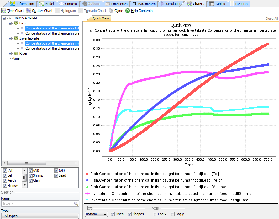 The plots of concentration in invertebrates should have been updated with the latest results. Let's add fish concentration to the plot as well:
- Expand the folder with today's date and the two children Fish and Invertebrate
- Select Concentration of the chemical in fish…. Keep the CTRL button on your keyboard pressed and select Concentration of the chemical in invertebrate…
- In the listings below, select all species of fish and all species of invertebrates.
- Below the plot, change the legend orientation to Bottom.
Does your plot resemble the picture on the right?
 Save as… button. Choose a name and folder for the project file and click Save.