
Table of Contents
Creating an aquatic food web - Tutorial
Purpose
The purpose of this tutorial is to get you acquainted with the MERLIN-Expo software. The situation is entirely fictitious, the data is fabricated.
Introduction
By using the aquatic food models you can design a full aquatic food web for a lake or river in the area you are studying. 1)
In this example we will create try to re-create a food web for the river Glein (on the mouth of which King Arthur had his first battle). During the battle there were severe cases of lead poisoning, and we will see if the fish diet of the soldiers was the cause. Three species of fish lived there: Eel, Perch and Minnow, and two species of invertebrates: Shrimp and Clams.
The tutorial consists of three parts. In this first part we will start small, with just a model for invertebrates. In part 2 we will add fish and a river. In part 3 we will add a human intake model as well as a model for man.
We will begin by creating a fresh project for use to work with. After, we will add a sub-system for the invertebrates. Next we select the contaminant we are interested in (lead) and add the organisms (invertebrates). After, we will look at some important input data sets and parameters. Finally we will run a simulation and check out the simulation results.
Step 1: Creating the project
In the Info screen, click the  New button. In the window that appears, choose the blank (empty) template. This will give us a clean canvas onto which we will paint our river and its inhabitants.
Step 2: Adding a model for invertebrates
We will now add a sub-system box for invertebrates. It is often (always) a good idea to start small and to build rather than adding all the sub-systems at once.
Go to the  Model screen. Right-click the empty area and choose Get from library…. A window appears with all the available sub-systems in the model library.

Locate and select the Invertebrate model. Click Ok. A single box should now appear in your graph. If you want to peek inside, click the + symbol.
Step 3: Selecting contaminants and species
Click the  Context tab.
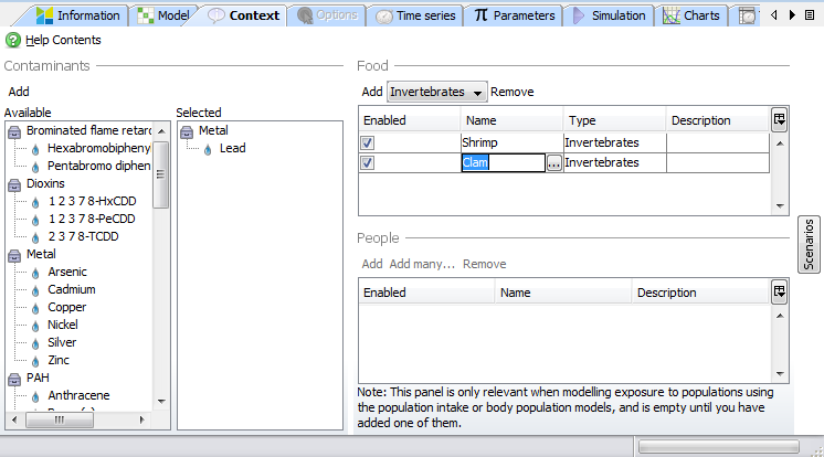
In the section named Contaminants, find Lead in the list and select it. It should now move from the 'available' to the 'selected' list.
In the Food section, there is a button named Add. Next to it is a drop-down list with available food types. The invertebrates sub-system offer just one food item type: invertebrate.
Click the Add button two times. Two items should now appear in the table below (Invertebrates and Invertebrates_2). Click in the Name cell of each to rename them to Shrimp and Clam.
Step 4: Adding time series input data
 There are only two important things to know about time series in MERLIN-Expo
- They start at day 0 2).
- The time unit is always days [d-1].
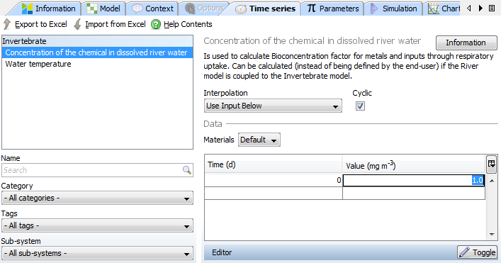
The invertebrates model require two (potentially) time dependent sets of data: concentration of the contaminant in water and the water temperature. We will let these be constant for now:
Click the  Time series tab. In the list both of the data items should be listed. Make sure that Concentration of the chemical in dissolved river water is selected. In the table, enter the value
| Time | Value [mg m-3] |
|---|---|
| 0.0 | 1.0 |
Next click Water temperature. Leave the value 15.0 as it is.
Step 5: Entering parameter values
 Proceed to the
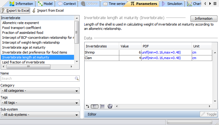
  Parameters screen. You might notice that it is very similar to the time series screen. The parameters are listed on the left hand side. When you select a parameter, the area to the right will display information and a table in which you can change the parameter data.
The table will (by default) show you the value, PDF and unit. The PDF is only relevant for probability studies and will be ignored in this exercise.
There are many parameters to find values for, and to keep you from getting bored we will only change a few of the parameters from their default values.
Invertibrate age at maturity
| Invertebrates | Value |
|---|---|
| Shrimp | 2200 |
| Clam | 1700 |
Invertebrate diet preference for food items - How much one species' diet consists of another species (cannibalism is also allowed).
| Invertebrates | Shrimp | Clam |
|---|---|---|
| Shrimp | 0 | 0.3 |
| Clam | 0 | 0 |
Invertebrate length at maturity
| Invertebrates | Value |
|---|---|
| Shrimp | 6 |
| Clam | 4 |
Step 6: Running a simulation
 Move on to the next tab,
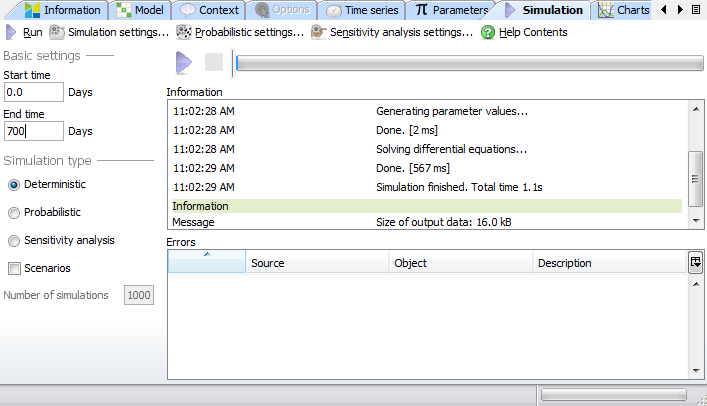
  Simulation. The simulation screen is were you make the final settings before performing a calculation. You specify the start and end time and what type of simulation you want to run. The
  Simulation Settings button allow you to select which data you want from the simulation and to play around with the solver settings.
Change the End time to 700 days, and then click the Run button to start the simulation. The Information area should now fill up with messages from the simulation engine.
Step 7: Plotting results
The reward of your labour is now within reach. Click the  Chart tab to access the charts screen. The chart screen and its close cousin, the
  tables screen, will list all the outputs of the simulation. Simulation results are overwritten each time you run a new simulation, but if you want to keep results - eg. to compare results from two different simulations - you can create archives of simulation data.
Expand the node with today's date, then expand the Invertebrates node.
Inside, click the Concentration of the chemical in invertebrates (…) label. This output will have different values for different species of invertebrates. If you had chosen to model more than one contaminant, it would also have different values for different contaminants. When you select the output, two lists should appear under it. One which lets you select species, one to select contaminants.
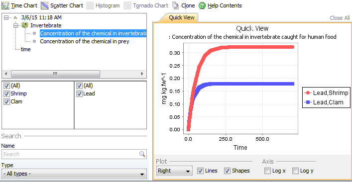 In the first list, select both Shrimp and Clam. A plot should now be displayed on the right hand side.
Below the graph are tools that can help modify the plot. Select a legend on the Right, and also check the Shapes box. The chart should resemble the picture on the right.
Step 8: Saving your project
Return to the Information tab. Click the  Save as… button. Choose a name and folder for the project file and click Save.
If you want to compare your results with ours, you can download the solution file here.
Are you ready to continue to part 2?